Fantasy Football with Scrapy and scikit-learn (Part 1)

The code for this project is available here: https://github.com/athompson1991/football. With this being my debut blog post, I’ve decided to break the analysis into two parts as there are many aspects to explain and the article getting to be a bit lengthy.

Intro

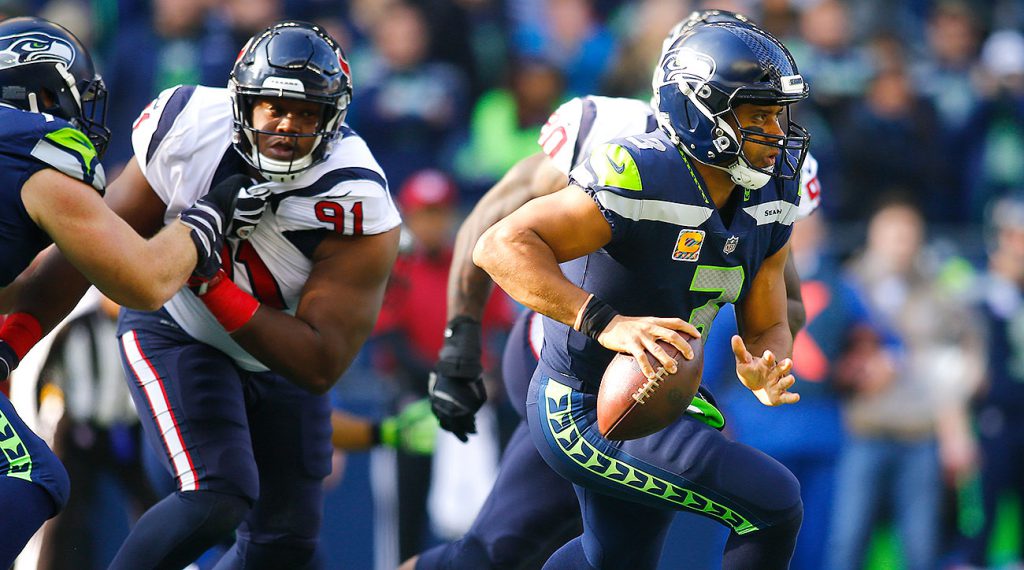
Football season has kicked off (pun intended), and likewise so has Fantasy football. I distinctly recall the last time I had a FF draft and how I essentially went in blind, with predictably mediocre results. This season, I wanted to Money Ball it using some machine learning techniques I acquired through classes at UW. Nothing particularly fancy, but enough to provide a semblance of judgement in picking my team.

As often happens with coding projects like this, I began with some scripts to get the data, followed by some scripts to do basic analysis, but the whole thing quickly metastasized into a larger endeavor. Ultimately the scraping work was consolidated into a module containing Scrapy spiders and pipelines/items/settings; the analysis section morphed into a more sophisticated object oriented approach to using scikit-learn; and the ultimate desire of a player ranking for the 2018 season was wrapped into an easily executable script.

Problem Scope

Before jumping into the actual project, I want to explain exactly how I approached this problem. There are important aspects of the Fantasy rules, the scraping, and the analysis that need to be considered.

My league is on Yahoo Fantasy Sports, and I had the following image as my guide on what the team would look like and how points would be gained:

A quick glance at this and a general understanding of football suggest how to launch the analysis: things like offensive fumble return TD or two point conversions can be ignored (very rare) and I can focus on yardage and touchdowns for passing/receiving/rushing (I also decide to predict total receptions for wide receivers).

Also note the make up of positions on the roster. While I could attempt to predict kickers, tight ends, and defense, I decide to simplify my analysis and focus exclusively on predicting the quarterback, wide receiver, and running back performance.

So, in summary, there will be seven response variables to predict (passing/receiving/rushing for TD and yardage, plus total receptions). That leaves the question of what the features will be. To answer this, we take a look at the Pro Football Reference website. Just as an example, take a look at the passing stats:

Many of these stats can be features, such as completion percentage, touchdown counts, and interception counts. Without looking at the stats for other positions (running back and wide receiver), we can kind of guess what will be useful: rushing yards, reception percentages, touchdown counts, etc. Anything numeric, really.

The trick is that we want to use last year’s stats to predict this year’s stats. This will involve a minor trick in Python, but is important to keep in mind. Obviously there is greater correlation between touchdowns and yardage in a given year than between touchdowns last year versus yardage this year.

Scraping

To get the data, I use the Python package Scrapy. Though this is not a tutorial specifically on how to use Scrapy, I will demonstrate the basic approach I took to go from scraping only the passing data, to using a more generalized means of scraping all player data.

Passing

Whenever I do a scraping project, I have to learn the inner workings of the HTML on the target website. For this, I simply looked up the passing stats for a given season, used the Scrapy shell to ping the website, then figured out exactly which cells/td elements to extract and how to do so.

As it turns out, the main table for the passing page is conveniently accessed using the CSS selector table#passing. You can see this by using the inspector in Chrome/Firefox:

Furthermore, all the data in the table is td elements (table data) nested in tr elements (table row). For my purposes, this means that my Scrapy spider will have to zero in on a row, then parse each data element cell by cell in that row. Instead of explaining all the minutia of how to do this, here is my first iteration of the spider to crawl the passing pages:

import scrapy
import bs4
from ..items import PassingItem

FOOTBALL_REFERENCE_URL = 'https://www.pro-football-reference.com'

class PassingSpider(scrapy.Spider):

    name = 'passing'
    allowed_domains = ['pro-football-reference.com']

    def __init__(self):
        super().__init__()
        self.years = list(range(1990, 2019))
        self.urls = [FOOTBALL_REFERENCE_URL + "/years/" + str(year) + "/passing.htm" for year in self.years]

    def parse_row(self, row):
        soup = bs4.BeautifulSoup(row.extract())
        tds = soup.find_all('td')
        if(len(tds) > 0):
            link = tds[0].find('a', href=True)['href']
            player_code = link.split('/')[-1]
            player_code = player_code[0:len(player_code) - 4]
            stats = {td["data-stat"]: td.text for td in tds}
            stats['player_code'] = player_code
            stats['player'] = stats['player'].replace('*', '')
            stats['player'] = stats['player'].replace('+', '')
            stats['pos'] = stats['pos'].upper()
            return stats
        else:
            return {}

    def parse(self, response):
        page = response.url
        self.log(page)
        passing = response.css("table#passing")
        passing_rows = passing.css('tr')
        for row in passing_rows[1:]:
            parsed_row = self.parse_row(row)
            if len(parsed_row) != 0:
                parsed_row['season'] = page.split('/')[-2]
                yield PassingItem(parsed_row)

    def start_requests(self):
        for url in self.urls:
            yield scrapy.Request(url=url, callback=self.parse)

The important lesson of this is that there is the primary parse method as well a parse_row helper method. A couple quick things to note:

  • The years I am pulling from are 1990 to 2019
  • BeautifulSoup is used to parse the HTML
  • Messy characters are removed
  • The neat trick to get all the data is on line 24, where I use a dictionary comprehension to pull every statistic in one fell swoop

I will not get into the Scrapy item or pipeline situation, but that is all available on my Github and there is Scrapy documentation is available for reference.

Generalizing for All Player Stats

Once I had written the passing spider, I moved on to get rushing statistics. However, I found myself writing an essentially identical spider. There were only two differences: the last part of the URL was “rushing” instead of “passing”, and the CSS selector was table#rushing instead of table#passing. This seemed like something which could easily be addressed and could avoid me a headache when I moved on to receiving as well.

My solution was inheritance. I wrapped the bulk of the code into a parent class PlayerSpider, then had the detailed particulars of each target page cooked into the inherited classes: PassingSpider, ReceivingSpider, RushingSpider, etc.

I wrote an inherited spider for (almost) all the pages listed under “Player Stats”

Without cluttering everything up with a giant Python class, the idea was to take the super class and base everything around the sub class name like so:

class PlayerSpider(scrapy.Spider):

    allowed_domains = ['pro-football-reference.com']

    def __init__(self, name):
        super().__init__()
        self.years = list(YEARS)
        self.urls = [FOOTBALL_REFERENCE_URL + "/years/" + str(year) + "/" + name + ".htm" for year in self.years]

...

    def parse(self, response, target, item_class):
        self.log("parsing row...")
        page = response.url
        table = response.css("table#" + target)
        table_rows = table.css('tr')
        for row in table_rows[1:]:
            parsed_row = self.parse_row(row)
            if len(parsed_row) != 0:
                parsed_row['season'] = page.split('/')[-2]
                yield item_class(parsed_row)

class PassingSpider(PlayerSpider):
    name = 'passing'

    def __init__(self):
        super().__init__(PassingSpider.name)

    def parse(self, response):
        return super().parse(response, target=PassingSpider.name, item_class=PassingItem)

The trick is in using the __init__ methods as a way to establish which page we are looking at, as well as what the table will be named (in other words, exactly the problem described above regarding passing versus rushing). The parsing methods on the parent class need to be modified slightly to account for more string manipulation issues, and the Scrapy item needs to be modified as well to adjust to different column headers, but otherwise the process is very similar for every statistic type (receiving, rushing, passing).

With some quick, additional Scrapy items and a CSV pipeline that spells out the columns to expect and where to save the data, I can easily pull all data of interest from 1990 to 2019: passing, rushing, receiving, defense, kicking, and fantasy.

With the “database” successfully established, we can now move on to the actual data analysis.

How I feel when I successfully scrape a bunch of data

Exploratory Data Analysis

With exploratory data analysis, I sought to do two things – manipulate the data into something that could be fed into a regression model, and get a cursory understanding of exactly what kind of relationships could be valuable.

Manipulating the Data

The idea of the predictions is to use present data to predict the next season’s performance. This is on an individual player level, and the type of performance (rushing, passing, receiving) is the basis of analysis.

To accomplish this, the underlying data has to be joined with itself – think of it as a SQL join where the column you are joining on is itself plus/minus one. The Python code is defined in the function make_main_df :

def make_main_df(filename):
    raw_data = pd.read_csv(filename)
    prev_season = raw_data.copy()
    prev_season['lookup'] = prev_season['season'] + 1
    main = pd.merge(
        raw_data,
        prev_season,
        left_on=['player_code', 'season'],
        right_on=['player_code', 'lookup'],
        suffixes=('_now', '_prev')
    )
    return main

Notice that the season field is joined on itself plus one and that the player_code is also part of the merge. The columns are renamed with suffixes that are self explanatory. If we use the Analyzer class I wrote for this project (more on that in the sequel to this blog post), we can see what kinds of columns this gives us for our analysis of passing data.

from football.analysis.analyzer import Analyzer

analyzer = Analyzer("script/analysis_config.json")
analyzer.set_analysis("passing")
analyzer.create_main_df()

analyzer.main.columns
 Index(['season_now', 'player_now', 'player_code', 'team_now', 'age_now',
        'pos_now', 'g_now', 'gs_now', 'qb_rec_now', 'pass_cmp_now',
        'pass_att_now', 'pass_cmp_perc_now', 'pass_yds_now', 'pass_td_now',
        'pass_td_perc_now', 'pass_int_now', 'pass_int_perc_now',
        'pass_long_now', 'pass_yds_per_att_now', 'pass_adj_yds_per_att_now',
        'pass_yds_per_cmp_now', 'pass_yds_per_g_now', 'pass_rating_now',
        'qbr_now', 'pass_sacked_now', 'pass_sacked_yds_now',
        'pass_net_yds_per_att_now', 'pass_adj_net_yds_per_att_now',
        'pass_sacked_perc_now', 'comebacks_now', 'gwd_now', 'season_prev',
        'player_prev', 'team_prev', 'age_prev', 'pos_prev', 'g_prev', 'gs_prev',
        'qb_rec_prev', 'pass_cmp_prev', 'pass_att_prev', 'pass_cmp_perc_prev',
        'pass_yds_prev', 'pass_td_prev', 'pass_td_perc_prev', 'pass_int_prev',
        'pass_int_perc_prev', 'pass_long_prev', 'pass_yds_per_att_prev',
        'pass_adj_yds_per_att_prev', 'pass_yds_per_cmp_prev',
        'pass_yds_per_g_prev', 'pass_rating_prev', 'qbr_prev',
        'pass_sacked_prev', 'pass_sacked_yds_prev', 'pass_net_yds_per_att_prev',
        'pass_adj_net_yds_per_att_prev', 'pass_sacked_perc_prev',
        'comebacks_prev', 'gwd_prev', 'lookup'],
       dtype='object')

Analyzing the Data

One thing that might be interesting to look at is the relationship between touchdowns and yardage. Is there any predictive power there?

Here is a plot of touchdown count versus yardage, per quarterback (so each dot is the quarterback, but any given quarterback could have many seasons plotted)

There is clearly a great relationship between these two variables (because obviously there would be). But do touchdowns this season provide any help in predicting next season‘s yardage? Here is that picture:

The relationship becomes much noisier. However, there does seem to be a nice, upward trend once the low touchdown/yardage observations are removed. If we filter results to “cleaner” quarterback observations, we get this plot:

This doesn’t look terrible! How does the current touchdown count versus next season’s touchdown count look?

Again, this is a filtered dataset and there does seem to be a degree of correlation present. If we plot the correlation matrix as a heatmap, we can get a better idea of exactly which of the variables available have predictive power and which do not.

There is a clear break between the “now” data and the “previous” data, as expected. However the large block in the middle of the triangle is of interest – this is what we will use to develop our models, and at first glance there does seem to be correlation.

I am going to leave the EDA at that because I could repeat this exercise for all the other positions and at the end of the day I am simply trying to use whatever is available to make an informed decision. The important conclusion from this analysis, though, is that there are quite a few numerical fields in each position to produce analysis and that, at first glance, there is reason to suspect something of value can be developed.

Conclusion

That’s all for now. I will explain the inner workings of my preprocessing, regressions, hyperparameter tuning, and predictions in the next post. I hope you found this overview of the web scraping and exploratory data analysis work useful and interesting!

Fantasy Football with Scrapy and scikit-learn (Part 2)

Welcome to part 2 of this tutorial! In the first part I went over how to get the data and do simple analysis, and in this section I will explain how I fit a number of different machine learning models. All of the code is available on Github.

Preprocessing and Pipelines

Now that the data has been acquired and determined to have predictive capabilities, we can turn our attention to building regression models. Before doing this, though, we want to make sure the data is clean, as well as in a proper format for model fitting.

For the purposes of this blog post, I’ll break the preprocessing into three components: filtering out dirty observations, calculating data standardization, and introducing polynomial features.

Filtering the Data

This is the simplest step in cleaning up the data, but it is certainly an important one. For example, with the raw passing data we only want to consider quarterbacks, but there are a number of different positions represented in the data set. Additionally, we want to filter down to those observations with a meaningful number of passes. The code ultimately looks like this:

print('prior shape: ' + str(main.shape[0]))
main = main[main['pass_att_prev'] > 100]
main = main[main['pass_att_now'] > 100]
main = main[main['pos_prev'] == 'QB']
print('post shape: ' + str(main.shape[0]))

The print commands are helpful in seeing just how much data is dropped, something always worth keeping in mind when doing statistical analysis.

I won’t repeat this for all the other positions, but a similar weeding out of bad data has to occur, obviously.

Standardization

Some regression/classification models (such as support vector machines) are sensitive to the scale of the data and need to have standardized observations in order to work properly. There are a few different ways to accomplish this, but here I will use the most common, which is to calculate the Z score (\frac{x-\mu}{\sigma}) of each observation.

This can be done using the StandardScaler class in scikit-learn. Though I skip directly to wrapping this scaler in a Pipeline (explained in the next section), the basic usage is something along the lines of:

from sklearn.preprocessing import StandardScaler
scaler = StandardScaler()
scaled_pass_att = scaler.fit_transform(main['pass_att_now'])

Polynomial Features

One thing to consider in modeling the data is the interaction between various features – perhaps player age and player interceptions aren’t significant features on their own, but age times interceptions is. From the scikit-learn documentation, if we have input features \mathbf{x}=[a, b] then the generated polynomial features (of degree 2) are \mathbf{x}=[1, a, b, a^2, ab, b^2]

This operation is accomplished simply using the PolynomialFeatures class in scikit-learn.

Pipelines

A helpful tool in the scikit-learn library is the Pipeline class. While each preprocessing step and model specification can be done one step at a time (by manually using the .fit_transform method), there is an alternative approach using pipelines.

Here, for example, is the first model I developed to predict passing yardage. I standardize the data, generate polynomial features, then fit a support vector regression (SVR) estimator

from sklearn.preprocessing import StandardScaler, PolynomialFeatures
from sklearn.model_selection import train_test_split
from sklearn.pipeline import Pipeline
from sklearn.svm import SVR

target = main['pass_yds_now']
features = main[[
    'age_prev',
    'pass_cmp_prev',
    'pass_att_prev',
    'pass_cmp_perc_prev',
    'pass_yds_prev',
    'pass_yds_per_att_prev',
    'pass_adj_yds_per_att_prev',
    'pass_yds_per_cmp_prev',
    'pass_yds_per_g_prev',
    'pass_net_yds_per_att_prev',
    'pass_adj_net_yds_per_att_prev',
    'pass_td_prev',
    'pass_td_perc_prev',
    'pass_int_prev',
    'pass_int_perc_prev',
    'pass_sacked_yds_prev',
    'pass_sacked_prev'
]]


features_train, features_test, target_train, target_test = train_test_split(features, target, test_size=0.2, random_state=42)


svr_pipeline = Pipeline([
    ('scaler', StandardScaler()),
    ('polyfeatures', PolynomialFeatures()),
    ('svr', SVR())
])

svr_pipeline.fit(features_train, target_train)

This is a useful way to avoid redundant code. Also, pipelines can be further complicated to address many other aspects of preprocessing and modeling, such as to calculate one-hot encoding or to impute missing values.

Fitting the Regression Models

I will attempt to very briefly explain the math behind these models and then demonstrate the code.

Regression Models

I decided to use three different regression techniques to predict the various target variables: support vector regression, random forest regression, and ridge regression. After fitting, then tuning the models, I effectively use a voting estimator and take an average of the three models to produce my player rankings.

Support Vector Machine

SVMs are often first explained in terms of the classifier. It is simply an optimization problem. The idea in classification is to draw a line (decision boundary) through the classes that maximizes the distance between them (the gap between the classes is sometimes referred to as the “street”); soft-margin classification relaxes the line-drawing so that the model is more flexible. With regression, the idea is the same but treats the street as a known distance/hyperparameter, \epsilon, and minimizes regression error such that the number of observations on the street is maximized. Without getting too deep into it, the optimization problem for soft margin support vector regression is

    \[\begin{array}{l r} \text{min} & \frac{1}{2}\mathbf{w}^T\mathbf{w}+C\sum_{i=1}^m\left(\zeta_i+\zeta_i^*\right)\\ \\ \text{s.t.} &  y_i - \mathbf{w}^T\mathbf{x}_i-b \leq \epsilon + \zeta_i\\ & \mathbf{w}^T\mathbf{x}_i + b - y_i \leq \epsilon + \zeta_i^* \\ & \zeta_i, \zeta_i^* \geq 0 \end{array}\]

where \mathbf{w} is the weight vector per feature, y_i is the known target variable, C is a regularization tuning variable, and \zeta_i,\zeta_i^* is a distance to the points outside the street.

There is also the kernel trick, which is a fancy way of transforming the training data without actually going through the trouble of doing the transform. For example, the kernel trick can be used to effectively recreate the polynomial features described previously:

    \[\phi(\mathbf{a})^T\phi(\mathbf{b})=\left(\mathbf{a}^T\mathbf{b}\right)^2\]

Random Forest Regression

Similar to the support vector machine, random forest models are typically explained as classification estimators. Random forest estimators are an extension of decision tree estimators. With decision trees, the idea is to minimize the Gini impurity in the training data:

    \[G_i=1-\sum_{j=1}^Np_{i,k}^2\]

Where p_{i, k} is the fraction of class k observations mislabeled as i. With random forests, many trees are generated and the training data is bootstrapped. We can easily go from classification to regression by predicting an individual value rather than a class.

Ridge Regression

While OLS linear regression is obviously the most common approach to regression, it is a model that is forced to utilize every feature to solve for the coefficients. Ridge regression is an interesting alternative which can discern between important features and less important one. The typical coefficient equation for OLS is

    \[\pmb{\hat{\beta}}=\left(\mathbf{X}^T\mathbf{X}\right)^{-1}\mathbf{X}^T\mathbf{Y}\]

Assuming \mathbf{X} is scaled, ridge regression incorporates a new hyperparameter, k, to “shrink” unimportant features and accentuate the more valuable data. The model becomes

    \[\pmb{\hat{\beta}}=\left(\mathbf{X}^T\mathbf{X}\right + k\mathbf{I})^{-1}\mathbf{X}^T\mathbf{Y}\]

Tuning the Models

The scikit-learn library allows us not to just fit the models, but also tune the various hyperparameters each may require. For example, ridge regression requires the variable k but it isn’t clear exactly what that value should be. To find this out, there are search classes available in scikit-learn that cross validate a grid of parameters and identify the best combination.

How to do it

To tune an estimator, you have a few options in scikit-learn. The two I know are GridSearchCV and RandomizedSearchCV, but others exist (such as a randomly sampled param grid). While the grid search is just that – a full search over the entire grid of parameters provided – the randomized search looks for better performing options and doesn’t try out every combination.

Though I ultimately ended up using the RandomizedSearchCV for the analysis, one of my old commits on Github utilized the GridSearchCV class like so (imports omitted, as well as the train/test split):

svr_pipeline = Pipeline([
    ('scaler', StandardScaler()),
    ('polyfeatures', PolynomialFeatures()),
    ('svr', SVR())
])


param_grid = [{
    'polyfeatures__degree': [1, 2, 3],
    'svr__epsilon': np.linspace(1, 1000, 10),
    'svr__kernel': ['linear', 'poly', 'sigmoid', 'rbf'],
    'svr__C': [0.1, 1, 10],
}]

grid_search = GridSearchCV(
    svr_pipeline,
    param_grid,
    cv=10,
    scoring='neg_mean_squared_error'
)

grid_search.fit(features_train, target_train)

There are a couple things to note. First, the syntax of the parameter grid – it is a dictionary of variables inside a list that get passed into the GridSearchCV class. Also note that the regression itself is built into a pipeline. What this means for the hyperparameter tuning is that the name of the pipe in the pipeline needs to be prefixed on the key of the param grid; notice that there is svr__epsilon in the param grid and that the corresponding tuple in the pipeline is named svr. Finally, it’s worth pointing out the argument cv in the grid search class means that there will be 10 fold cross validation and that the scoring argument is negative mean squared error (a typical scoring calculation for regression problems).

Once the grid search works out the best model, you can easily retrieve it for further analysis

from sklearn.metrics import mean_squared_error
from sklearn.model_selection import cross_val_predict

best_model = grid_search.best_estimator_
predictions = cross_val_predict(
    best_model,
    features_train,
    target_train,
    cv=10
)
score = np.sqrt(mean_squared_error(predictions, target_train))
print('Grid Search SVR MSE: ' + str(score))

Example: Tuning the Ridge Regression to Address Overfitting

As noted earlier, the k parameter of the ridge regression can be tuned. In the case of this project, the first model I fit has the passing touchdowns this season as the target variable and uses 17 features from the previous season as input.

Let’s take a look at the learning curve for the raw, untuned model.

The orange line is the out of sample prediction and the blue line is the in sample; so, in-sample the model predicts with 400 observations, on average, an error of about eight touchdowns, and out-of-sample an average error of about nine. The large gap between these two lines suggests the model is overfitting. Can this be fixed by tuning the k value? Here is what the learning curve looks like with the tuned model using randomized search

Clearly the model is improved and the gap between the two lines is significantly reduced (though, honestly, an error rate of 8 touchdowns is rather large and the more serious problem here is underfitting)

Bringing it All Together

So now we have all the steps of the analysis outlined

  1. Manipulate the data into the format we want
  2. Filter down the observations into a clean dataset
  3. Specify and fit the models
  4. Tune the hyperparameters for every model
  5. Make predictions about this season

And this has to be done 7 times for various different metrics. Instead of writing a script line-by-line, I have built out a class, Analyzer, to execute all of these steps. All the functionality of the machine learning is simply wrapped in that class, and (for now) it is assumed that the code will be executed in order.

Configuration

Since the process is quite similar for every analysis, I thought it would be prudent to put the model specifications into a JSON file. This way, if I need to change, say, the target variable then I can simply change the code in the configuration file rather than having to root through a large script or Jupyter notebook.

The JSON analysis specs look like this

{
  "home_dir": "./",

  "passing_analysis": {
    "main_df": "data/passing.csv",
    "target": "pass_td_now",
    "features": [
      "age_prev",
      "pass_cmp_prev",
      "pass_att_prev",
      "pass_cmp_perc_prev",
      "pass_yds_prev",
      "pass_yds_per_att_prev",
      "pass_adj_yds_per_att_prev",
      "pass_yds_per_cmp_prev",
      "pass_yds_per_g_prev",
      "pass_net_yds_per_att_prev",
      "pass_adj_net_yds_per_att_prev",
      "pass_td_prev",
      "pass_td_perc_prev",
      "pass_int_prev",
      "pass_int_perc_prev",
      "pass_sacked_yds_prev",
      "pass_sacked_prev"
    ],
    "filters": [
      ["pass_att_prev", ">",  100],
      ["pass_att_now", ">", 100],
      ["pos_prev", "==", "'QB'"]
    ],
    "hypertune_params": {
      "search_class": "RandomizedSearchCV",
      "cv": 10,
      "scoring": "neg_mean_squared_error"
    },
    "models": {
      "support_vector_machine": {
        "pipeline": {
          "scaler": "StandardScaler",
          "poly_features": "PolynomialFeatures",
          "svr": "SVR"
        },
        "search_params": {
          "poly_features__degree": [1, 2, 3],
          "svr__kernel": ["linear", "rbf", "sigmoid"],
          "svr__epsilon": [0.5, 1, 1.5]
        }
      },
      "random_forest_regressor": {
        "pipeline": {
          "scaler": "StandardScaler",
          "poly_features": "PolynomialFeatures",
          "random_forest": "RandomForestRegressor"
        },
        "search_params": {
          "poly_features__degree": [1, 2],
          "random_forest__max_depth": [2, 3, 5, 1000],
          "random_forest__min_samples_leaf": [1, 10, 20, 40, 60, 80, 100]
        }
      },
      "ridge": {
        "pipeline": {
          "scaler": "StandardScaler",
          "poly_features": "PolynomialFeatures",
          "ridge_regression": "Ridge"
        },
        "search_params": {
          "poly_features__degree": [1, 2, 3],
          "ridge_regression__alpha": [0.1, 0.2, 0.3, 0.4, 0.5]
        }
      }
    }
  }
}

This spells out the whole process! The CSV we want? It’s located in data/passing.csv. The filters? They’re specified under “filters”. Add or drop features? Easy. The models are a little tricky in how they are configured, but it is exactly the same process as before – it requires that any modeling be done using a pipeline, but then the parameter grid for tuning can be changed quite easily.

Additional analysis specifications can be inserted into this as well, as long as they have a similar _analysis suffix.

Execution in Python

It is simple to take this configuration and actually execute the scikit-learn code.

analyzer = Analyzer("config.json")
analyzer.set_analysis("passing")
analyzer.create_main_df()
analyzer.filter_main()
analyzer.split_data()
analyzer.create_models()
analyzer.run_models()
analyzer.tune_models()

This will run all the steps listed in the config file. I want to build out unit tests for this class to guarantee it handles everything as expected, but for the purposes of this analysis the code does work as intended.

Prediction

Now to finally get the power rankings.

Assume that the config file spells out all seven target variables we want and how to run the regressions on them. Assume that the Analyzer class has done all the hard work of preprocessing, model fitting, and model tuning.

Now, we want to take the original dataset, put the suffix _prev onto the 2018 season data, then use that as the input into the Analyzer instance to get the prediction of each metric (passing/receiving/rushing stats on touchdowns and yardage, plus total receptions).

This seemingly tricky operation can be done using the following function

def predict_from_raw(main, analyzer):
    df = main.copy()
    df.columns = [col + "_prev" for col in df.columns]
    features = df[analyzer.features_names]
    predictions = analyzer.predict_tuned_models(features)
    names = df["player_prev"]
    names.index = range(len(names))
    predictions['name'] = names
    return predictions

Notice the method .predict_tuned_models. This is what will run a prediction based on the input data for each model from the configuration file.

Once all the predictions have been made, we want to take the predicted statistic and calculate the corresponding fantasy points

models = ['support_vector_machine', 'random_forest_regressor', 'ridge']
passing_fantasy_yds = passing_yds_predictions[models].div(25)
receiving_fantasy_yds = receiving_yds_predictions[models].div(10)
rushing_fantasy_yds = rushing_yds_predictions[models].div(10)

passing_fantasy_td = passing_td_predictions[models].mul(4)
receiving_fantasy_td = receiving_td_predictions[models].mul(6)
rushing_fantasy_td = rushing_td_predictions[models].mul(6)

receiving_fantasy_rec = receiving_rec_predictions[models]

Now that all the predictions have been made and turned into fantasy points, the last step is to take an average of each model for an overall ranking (this function is admittedly pretty hacky to get the receptions shoehorned in there but gets the job done for now).

def get_ranking(yds, td, main_df, rec=None):
    vote_yds = yds.apply(np.mean, axis=1)
    vote_yds.index = main_df['player_code']
    vote_td = td.apply(np.mean, axis=1)
    vote_td.index = main_df['player_code']
    if rec is not None:
        vote_rec = rec.apply(np.mean, axis=1)
        vote_rec.index = main_df['player_code']
        vote = vote_yds + vote_td + vote_rec
    else:
        vote = vote_yds + vote_td
    return vote

Results

And here are the results!

QB

pointspositionplayer
MahoPa00313.14238QBPatrick Mahomes
LuckAn00295.370346QBAndrew Luck
RoetBe00289.55698QBBen Roethlisberger
RyanMa00273.549325QBMatt Ryan
GoffJa00267.91081QBJared Goff
CousKi00263.739173QBKirk Cousins
BreeDr00262.422544QBDrew Brees
BradTo00249.018828QBTom Brady
MayfBa00246.809009QBBaker Mayfield
RivePh00246.742789QBPhilip Rivers

WR

pointspositionplayer
HopkDe00265.0243634WRDeAndre Hopkins
JoneJu02263.8836521WRJulio Jones
AdamDa01257.2140158WRDavante Adams
BrowAn04252.9623443WRAntonio Brown
ThomMi05250.3592538WRMichael Thomas
SmitJu00244.594075WRJuJu Smith-Schuster
ThieAd00241.9040111WRAdam Thielen
HillTy00240.7230349WRTyreek Hill
EvanMi00233.97766WRMike Evans
HiltT.00215.3827413WRT.Y. Hilton

RB

pointspositionplayer
GurlTo01176.535942RBTodd Gurley
ElliEz00156.799343RBEzekiel Elliott
BarkSa00150.807151RBSaquon Barkley
MixoJo00145.69819RBJoe Mixon
ConnJa00143.190105RBJames Conner
CarsCh00137.216166RBChris Carson
GordMe00136.926972RBMelvin Gordon
MackMa00135.825863RBMarlon Mack
HuntKa00127.118146RBKareem Hunt
McCaCh01125.465541RBChristian McCaffrey

A quick comment on trying to recreate these results: a lot of the methods in the machine learning algorithms employ randomness (stochastic gradient descent, the random forests algo, etc), so unless you carefully set a seed you may (read: will) see slightly different rankings.

Conclusions

The Good

I like that my number one QB ranking was Mahomes and that number two was Andrew Luck! This suggests that at least something was right with my models! The little I did know going into this season was that Mahomes was highly regarded (first round pick) and that Andrew Luck was also considered quite valuable (until, uh, recently). On the whole, I think the analysis gave me what I wanted: a generally more coherent approach to picking a fantasy team than randomly guessing.

I also like that the configuration file is in JSON and seems pretty extensible. I would like to build out more functionality for plotting capabilities and think it would even be cool to get a front end that runs the Python on the fly in the background and perhaps is accessed through a REST service. I think that the Analyzer class can be utilized for other CSV files as well, or perhaps have a database connection, and there is potential for building out more functionality in general.

The Bad

I do not like that my number three QB ranking was Ben Rothlisberger! That totally torpedoed my team last week! Though this analysis provides a better-than-totally-random picking ability, it does not give a super precise prediction – recall that the ridge model was underfitting. There is obviously a whole universe of analysis dedicated to figuring this stuff out, but needless to say more can be done than what I worked out here.

Another notable absence is any way to go about drafting the players based on this data. Though I can see the top predicted performance, there isn’t any optimization that provides me a list of who to pick in the draft and which round – Mahomes was taken immediately and wide receivers were the next fastest to be removed. How to account for this? My guess is some kind of constrained linear optimization problem, which perhaps can be another project.

The Ugly

I do not like that the Analyzer class is untested. This isn’t a crisis for this first pass, but it is something I would like to clean up. Additionally, the regression estimator classes from scikit-learn (Ridge, SVR, and RandomForestRegressor) have been imported manually into the Python module that establishes the Analyzer class, which is not ideal. I would like to have a way to lookup the regressors dynamically, so that other regressors from scikit-learn (such as Lasso or BaggingRegressor) can be incorporated.

Final Note

That’s it! I hope you found this analysis interesting! I hope that somebody reads this!

This is my first blog post ever on anything related to data science or coding, so I am certainly open to suggestions on how to better present my work. Let me know in the comments, or by email.

I do intend on developing this further and so some of the conclusions in this post may be different going forward, but otherwise this should be a pretty good overview of this entire project.

Have a nice day!