Genetic Algorithm for Simple Linear Regression

The basic idea of a genetic algorithm (GA) is to simulate the natural process of evolution and utilize it as a means of estimating an optimal solution. There are many applications of this technique, one of which being a fascinating YouTube video of a genetic algorithm that plays Mario. Yesterday I was wondering to myself if I could implement one for the (much) simpler task of estimating coefficients in a linear regression, and by midnight I had successfully written the Python code to accomplish this task.

All code can be found here on my Github.

General Idea

I’ve looked into GAs in the past, so I have a basic idea of the steps involved:

1. Initialize
2. Selection
3. Crossover
4. Repeat

As I mentioned, the idea is to resemble actual evolution, which is where these steps come from. First, you initialize your population: Adam and Eve (but in our case this will be ten thousand standard normal observations). Of that population, you evaluate “fitness” using some measure, and then cull the herd to those which are most fit – survival of the fittest, literally. Using the reduced population, you then breed them and add some genetic variation. This gives you the next “generation” of observations for which you repeat the selection and crossover process until you achieve your optimal solution.

Problem Statement

Because a GA is an optimization technique, there are many practical applications of the method (for example, the knapsack problem). However, I wanted to keep it simple – estimate the coefficients in a linear regression. As we all know, the general formula for a linear regression is:

The coefficients are picked to minimize the residual sum of squares (RSS). Estimates of the unknown coefficients are calculated like so:

I arbitrarily picked a specific true equation for simulation:

Here is the code to generate the data:

import numpy as np
import matplotlib.pyplot as plt
from sklearn.linear_model import LinearRegression
from sklearn.metrics import mean_squared_error, mean_absolute_error

np.random.seed(8675309)
x1 = np.random.normal(loc=2, scale=3, size=1000)
x2 = np.random.normal(loc=-1, scale=2, size=1000)
x = np.column_stack((x1, x2))
y = 3 * x1 + -4 * x2 + np.random.normal(size=1000)

Using linear regression from scikit-learn, we can easily see the coefficients are estimated as anticipated:

linear_regression = LinearRegression()
linear_regression.fit(x, y)
print(linear_regression.coef_)
[ 2.99810571 -3.98150108]

We can take a quick look at the mean squared error (MSE) and mean absolute error (MAE) of the fitted regression model:

y_hat = linear_regression.predict(x)

mean_squared_error(y, y_hat)
1.013983786908985

mean_absolute_error(y, y_hat)
0.8056630814774554

Now, we want to see what happens when we produce the same estimate using a genetic algorithm implementation.

Genetic Algo Technique

The first step is initialization. What this means in this context is a guess of coefficient pairs where is the population size of a generation (ten thousand, in this exercise) and is the number of coefficients to be estimated (two). Additionally, I define the fitness function to be optimized, which in this case is MSE.

def fitness(c):
    y_hat = np.dot(x, c)
    return mean_squared_error(y, y_hat)

n_epochs = 8
pop = 10000

# Here are the initialized guesses:
coefs = np.column_stack([np.random.normal(size=pop) for i in range(m)])

With these coefficients, we can produce a scatter plot of each pair’s fitness using a color gradient (greener has lower MSE). The “X” marks the true coefficient pair:

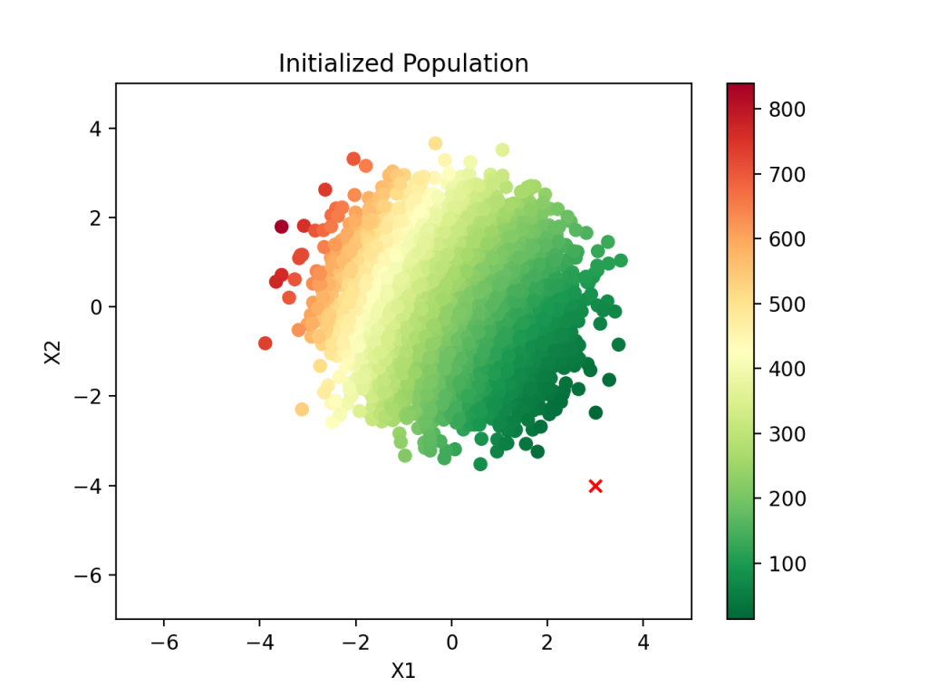
As we can see, there is a clear direction for the population to go in that will move it toward the target. Also, notice that the typical MSE is somewhere between 100 and 1000, which is wildly greater (worse) than the optimal MSE of 1. Clearly there is a lot of room for improvement over randomly guessing the coefficients.

We have initialized the population and can therefore execute the selection phase. We simple do away with the less fit population, keeping only the top 25% observations:

Now comes crossover. With 25% of the population remaining, we pair the observations and produce “children” of the pairs. This means that for each pair of “parents”, eight children are required to get a population with the original size of ten thousand. To guarantee the children do not all have the same midpoint value, I add some noise with numpy, which represents the “genetic variation” component of this analysis.

Once crossover is complete and the population returns to its original ten thousand, repeat selection and crossover until the optimal solution is achieved. This is the code which runs this process:

for epoch in range(n_epochs):
    culling = pop // 4
    f_hat = np.apply_along_axis(fitness, 1, coefs)
    df = np.append(coefs, f_hat.reshape(-1, 1), axis=1)
    df_sorted = df[np.argsort(df[:, m])]

    # Selection: survival of the fittest
    keep = df_sorted[0:culling]
    best = keep[0]
    print(f"Epoch: {epoch + 1}, Average fitness: {np.mean(keep[0, m]):.{4}f}, "
          f"Best X1: {best[0]:.{4}f}, Best X2: {best[1]:.{4}f}")

    new_coefs = []
    for i in range(0, culling, 2):
        mids = []
        for k in range(m):

            # Crossover: midpoint of coefficient pair

            mids.append((keep[i, k] + keep[i + 1, k]) / 2)
        for j in range(8):

            # Mutation: Add some noise to the result

            mutate_mids = [mid + np.random.normal() for mid in mids]
            new_coefs.append(mutate_mids)
    coefs = new_coefs

Here is the output from that code:

Epoch: 1, Average fitness: 13.2631, Best X1: 3.0064, Best X2: -2.3699
Epoch: 2, Average fitness: 1.0731, Best X1: 2.9791, Best X2: -4.1012
Epoch: 3, Average fitness: 1.0348, Best X1: 2.9761, Best X2: -3.9739
Epoch: 4, Average fitness: 1.0269, Best X1: 2.9816, Best X2: -4.0109
Epoch: 5, Average fitness: 1.0177, Best X1: 3.0099, Best X2: -3.9948
Epoch: 6, Average fitness: 1.0179, Best X1: 3.0039, Best X2: -3.9924
Epoch: 7, Average fitness: 1.0209, Best X1: 3.0190, Best X2: -4.0087
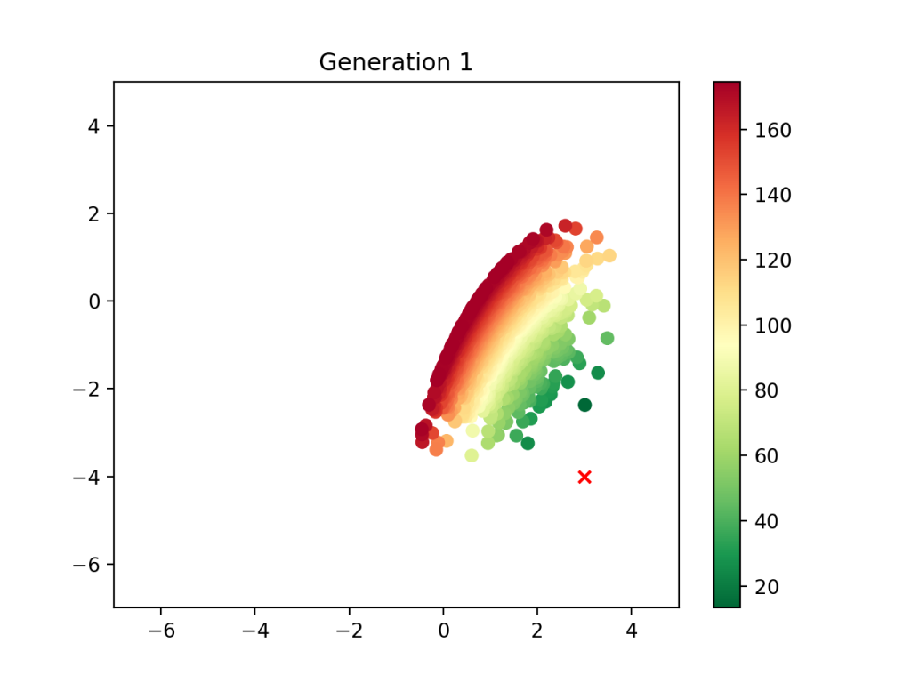
Epoch: 8, Average fitness: 1.0185, Best X1: 3.0136, Best X2: -3.9797

The average MSE drops substantially after just one generation and quickly settles into the minimal value determined previously by OLS linear regression. By the third generation, the best estimate is very near the true coefficient. As before, we can visualize this process at each step:

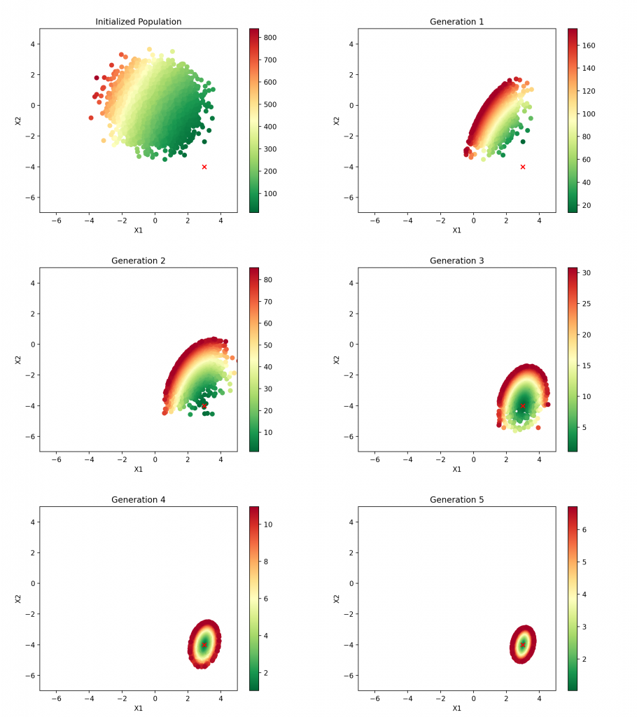
Clearly the population gravitates toward the correct answer. Subsequent generations are identical to generation five, and the optimal solution is identified.

Conclusion

This is certainly a toy example and not particularly useful, but the process of using a GA for optimization is nonetheless interesting to explore. Just from this example, there are several obvious concepts which can be further investigated: analysis of population size and culling percentage (hyperparameter tuning), trying the GA on a more complex regression model, when to stop the algorithm, etc. The OLS linear regression closed solution estimate is much faster to calculate than this GA trick, so performance is not gained in this toy example over the good, old-fashioned OLS linear regression.

Finally, I’ll also note that on a basic level my motivation for looking into this is that evolution in the real world is amazing and can produce optimal results that are mind blowing. For example, hummingbirds are so effective at flight that they resemble drones to me, some of the most cutting edge flight technology in the modern world. Also interesting is that there are many suboptimal outcomes, such as the existence of the seemingly useless appendix organ. It’s all quite strange. The fact that I can implement a similar process using Python and, in seconds, run my own quasi-evolutionary simulation is very cool to me.