Fantasy Football with Scrapy and scikit-learn (Part 2)

Welcome to part 2 of this tutorial! In the first part I went over how to get the data and do simple analysis, and in this section I will explain how I fit a number of different machine learning models. All of the code is available on Github.

Preprocessing and Pipelines

Now that the data has been acquired and determined to have predictive capabilities, we can turn our attention to building regression models. Before doing this, though, we want to make sure the data is clean, as well as in a proper format for model fitting.

For the purposes of this blog post, I’ll break the preprocessing into three components: filtering out dirty observations, calculating data standardization, and introducing polynomial features.

Filtering the Data

This is the simplest step in cleaning up the data, but it is certainly an important one. For example, with the raw passing data we only want to consider quarterbacks, but there are a number of different positions represented in the data set. Additionally, we want to filter down to those observations with a meaningful number of passes. The code ultimately looks like this:

print('prior shape: ' + str(main.shape[0]))
main = main[main['pass_att_prev'] > 100]
main = main[main['pass_att_now'] > 100]
main = main[main['pos_prev'] == 'QB']
print('post shape: ' + str(main.shape[0]))

The print commands are helpful in seeing just how much data is dropped, something always worth keeping in mind when doing statistical analysis.

I won’t repeat this for all the other positions, but a similar weeding out of bad data has to occur, obviously.

Standardization

Some regression/classification models (such as support vector machines) are sensitive to the scale of the data and need to have standardized observations in order to work properly. There are a few different ways to accomplish this, but here I will use the most common, which is to calculate the Z score ( $\frac{x-\mu}{\sigma}$ ) of each observation.

This can be done using the StandardScaler class in scikit-learn. Though I skip directly to wrapping this scaler in a Pipeline (explained in the next section), the basic usage is something along the lines of:

from sklearn.preprocessing import StandardScaler
scaler = StandardScaler()
scaled_pass_att = scaler.fit_transform(main['pass_att_now'])

Polynomial Features

One thing to consider in modeling the data is the interaction between various features – perhaps player age and player interceptions aren’t significant features on their own, but age times interceptions is. From the scikit-learn documentation, if we have input features $\mathbf{x}=[a, b]$ then the generated polynomial features (of degree 2) are $\mathbf{x}=[1, a, b, a^2, ab, b^2]$

This operation is accomplished simply using the PolynomialFeatures class in scikit-learn.

Pipelines

A helpful tool in the scikit-learn library is the Pipeline class. While each preprocessing step and model specification can be done one step at a time (by manually using the .fit_transform method), there is an alternative approach using pipelines.

Here, for example, is the first model I developed to predict passing yardage. I standardize the data, generate polynomial features, then fit a support vector regression (SVR) estimator

from sklearn.preprocessing import StandardScaler, PolynomialFeatures
from sklearn.model_selection import train_test_split
from sklearn.pipeline import Pipeline
from sklearn.svm import SVR

target = main['pass_yds_now']
features = main[[
    'age_prev',
    'pass_cmp_prev',
    'pass_att_prev',
    'pass_cmp_perc_prev',
    'pass_yds_prev',
    'pass_yds_per_att_prev',
    'pass_adj_yds_per_att_prev',
    'pass_yds_per_cmp_prev',
    'pass_yds_per_g_prev',
    'pass_net_yds_per_att_prev',
    'pass_adj_net_yds_per_att_prev',
    'pass_td_prev',
    'pass_td_perc_prev',
    'pass_int_prev',
    'pass_int_perc_prev',
    'pass_sacked_yds_prev',
    'pass_sacked_prev'
]]


features_train, features_test, target_train, target_test = train_test_split(features, target, test_size=0.2, random_state=42)


svr_pipeline = Pipeline([
    ('scaler', StandardScaler()),
    ('polyfeatures', PolynomialFeatures()),
    ('svr', SVR())
])

svr_pipeline.fit(features_train, target_train)

This is a useful way to avoid redundant code. Also, pipelines can be further complicated to address many other aspects of preprocessing and modeling, such as to calculate one-hot encoding or to impute missing values.

Fitting the Regression Models

I will attempt to very briefly explain the math behind these models and then demonstrate the code.

Regression Models

I decided to use three different regression techniques to predict the various target variables: support vector regression, random forest regression, and ridge regression. After fitting, then tuning the models, I effectively use a voting estimator and take an average of the three models to produce my player rankings.

Support Vector Machine

SVMs are often first explained in terms of the classifier. It is simply an optimization problem. The idea in classification is to draw a line (decision boundary) through the classes that maximizes the distance between them (the gap between the classes is sometimes referred to as the “street”); soft-margin classification relaxes the line-drawing so that the model is more flexible. With regression, the idea is the same but treats the street as a known distance/hyperparameter, $\epsilon$ , and minimizes regression error such that the number of observations on the street is maximized. Without getting too deep into it, the optimization problem for soft margin support vector regression is

$\begin{array}{l r} \text{min} & \frac{1}{2}\mathbf{w}^T\mathbf{w}+C\sum_{i=1}^m\left(\zeta_i+\zeta_i^*\right)\\ \\ \text{s.t.} & y_i - \mathbf{w}^T\mathbf{x}_i-b \leq \epsilon + \zeta_i\\ & \mathbf{w}^T\mathbf{x}_i + b - y_i \leq \epsilon + \zeta_i^* \\ & \zeta_i, \zeta_i^* \geq 0 \end{array}$

where $\mathbf{w}$ is the weight vector per feature, $y_i$ is the known target variable, $C$ is a regularization tuning variable, and $\zeta_i,\zeta_i^*$ is a distance to the points outside the street.

There is also the kernel trick, which is a fancy way of transforming the training data without actually going through the trouble of doing the transform. For example, the kernel trick can be used to effectively recreate the polynomial features described previously:

$\phi(\mathbf{a})^T\phi(\mathbf{b})=\left(\mathbf{a}^T\mathbf{b}\right)^2$

Random Forest Regression

Similar to the support vector machine, random forest models are typically explained as classification estimators. Random forest estimators are an extension of decision tree estimators. With decision trees, the idea is to minimize the Gini impurity in the training data:

$G_i=1-\sum_{j=1}^Np_{i,k}^2$

Where $p_{i, k}$ is the fraction of class $k$ observations mislabeled as $i$ . With random forests, many trees are generated and the training data is bootstrapped. We can easily go from classification to regression by predicting an individual value rather than a class.

Ridge Regression

While OLS linear regression is obviously the most common approach to regression, it is a model that is forced to utilize every feature to solve for the coefficients. Ridge regression is an interesting alternative which can discern between important features and less important one. The typical coefficient equation for OLS is

$\pmb{\hat{\beta}}=\left(\mathbf{X}^T\mathbf{X}\right)^{-1}\mathbf{X}^T\mathbf{Y}$

Assuming $\mathbf{X}$ is scaled, ridge regression incorporates a new hyperparameter, $k$ , to “shrink” unimportant features and accentuate the more valuable data. The model becomes

$\pmb{\hat{\beta}}=\left(\mathbf{X}^T\mathbf{X}\right + k\mathbf{I})^{-1}\mathbf{X}^T\mathbf{Y}$

Tuning the Models

The scikit-learn library allows us not to just fit the models, but also tune the various hyperparameters each may require. For example, ridge regression requires the variable $k$ but it isn’t clear exactly what that value should be. To find this out, there are search classes available in scikit-learn that cross validate a grid of parameters and identify the best combination.

How to do it

To tune an estimator, you have a few options in scikit-learn. The two I know are GridSearchCV and RandomizedSearchCV, but others exist (such as a randomly sampled param grid). While the grid search is just that – a full search over the entire grid of parameters provided – the randomized search looks for better performing options and doesn’t try out every combination.

Though I ultimately ended up using the RandomizedSearchCV for the analysis, one of my old commits on Github utilized the GridSearchCV class like so (imports omitted, as well as the train/test split):

svr_pipeline = Pipeline([
    ('scaler', StandardScaler()),
    ('polyfeatures', PolynomialFeatures()),
    ('svr', SVR())
])


param_grid = [{
    'polyfeatures__degree': [1, 2, 3],
    'svr__epsilon': np.linspace(1, 1000, 10),
    'svr__kernel': ['linear', 'poly', 'sigmoid', 'rbf'],
    'svr__C': [0.1, 1, 10],
}]

grid_search = GridSearchCV(
    svr_pipeline,
    param_grid,
    cv=10,
    scoring='neg_mean_squared_error'
)

grid_search.fit(features_train, target_train)

There are a couple things to note. First, the syntax of the parameter grid – it is a dictionary of variables inside a list that get passed into the GridSearchCV class. Also note that the regression itself is built into a pipeline. What this means for the hyperparameter tuning is that the name of the pipe in the pipeline needs to be prefixed on the key of the param grid; notice that there is svr__epsilon in the param grid and that the corresponding tuple in the pipeline is named svr. Finally, it’s worth pointing out the argument cv in the grid search class means that there will be 10 fold cross validation and that the scoring argument is negative mean squared error (a typical scoring calculation for regression problems).

Once the grid search works out the best model, you can easily retrieve it for further analysis

from sklearn.metrics import mean_squared_error
from sklearn.model_selection import cross_val_predict

best_model = grid_search.best_estimator_
predictions = cross_val_predict(
    best_model,
    features_train,
    target_train,
    cv=10
)
score = np.sqrt(mean_squared_error(predictions, target_train))
print('Grid Search SVR MSE: ' + str(score))

Example: Tuning the Ridge Regression to Address Overfitting

As noted earlier, the $k$ parameter of the ridge regression can be tuned. In the case of this project, the first model I fit has the passing touchdowns this season as the target variable and uses 17 features from the previous season as input.

Let’s take a look at the learning curve for the raw, untuned model.

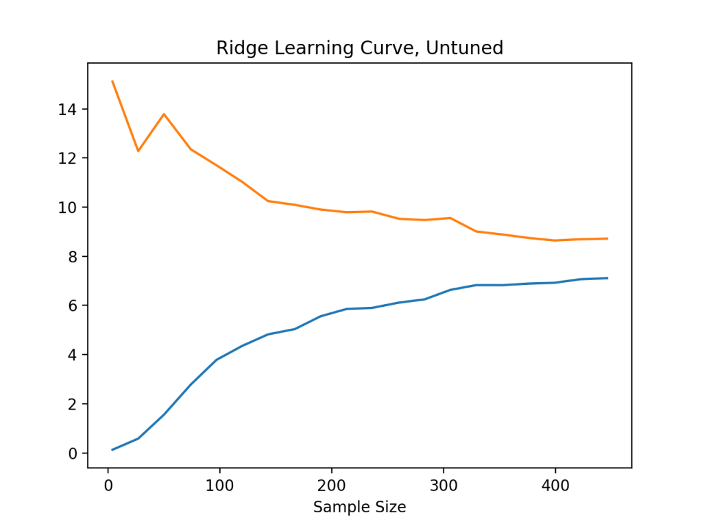
The orange line is the out of sample prediction and the blue line is the in sample; so, in-sample the model predicts with 400 observations, on average, an error of about eight touchdowns, and out-of-sample an average error of about nine. The large gap between these two lines suggests the model is overfitting. Can this be fixed by tuning the $k$ value? Here is what the learning curve looks like with the tuned model using randomized search

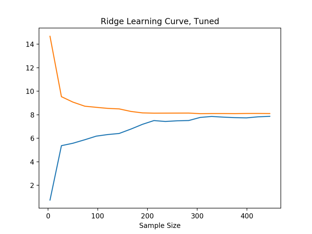
Clearly the model is improved and the gap between the two lines is significantly reduced (though, honestly, an error rate of 8 touchdowns is rather large and the more serious problem here is underfitting)

Bringing it All Together

So now we have all the steps of the analysis outlined

Manipulate the data into the format we want
Filter down the observations into a clean dataset
Specify and fit the models
Tune the hyperparameters for every model
Make predictions about this season

And this has to be done 7 times for various different metrics. Instead of writing a script line-by-line, I have built out a class, Analyzer, to execute all of these steps. All the functionality of the machine learning is simply wrapped in that class, and (for now) it is assumed that the code will be executed in order.

Configuration

Since the process is quite similar for every analysis, I thought it would be prudent to put the model specifications into a JSON file. This way, if I need to change, say, the target variable then I can simply change the code in the configuration file rather than having to root through a large script or Jupyter notebook.

The JSON analysis specs look like this

{
  "home_dir": "./",

  "passing_analysis": {
    "main_df": "data/passing.csv",
    "target": "pass_td_now",
    "features": [
      "age_prev",
      "pass_cmp_prev",
      "pass_att_prev",
      "pass_cmp_perc_prev",
      "pass_yds_prev",
      "pass_yds_per_att_prev",
      "pass_adj_yds_per_att_prev",
      "pass_yds_per_cmp_prev",
      "pass_yds_per_g_prev",
      "pass_net_yds_per_att_prev",
      "pass_adj_net_yds_per_att_prev",
      "pass_td_prev",
      "pass_td_perc_prev",
      "pass_int_prev",
      "pass_int_perc_prev",
      "pass_sacked_yds_prev",
      "pass_sacked_prev"
    ],
    "filters": [
      ["pass_att_prev", ">",  100],
      ["pass_att_now", ">", 100],
      ["pos_prev", "==", "'QB'"]
    ],
    "hypertune_params": {
      "search_class": "RandomizedSearchCV",
      "cv": 10,
      "scoring": "neg_mean_squared_error"
    },
    "models": {
      "support_vector_machine": {
        "pipeline": {
          "scaler": "StandardScaler",
          "poly_features": "PolynomialFeatures",
          "svr": "SVR"
        },
        "search_params": {
          "poly_features__degree": [1, 2, 3],
          "svr__kernel": ["linear", "rbf", "sigmoid"],
          "svr__epsilon": [0.5, 1, 1.5]
        }
      },
      "random_forest_regressor": {
        "pipeline": {
          "scaler": "StandardScaler",
          "poly_features": "PolynomialFeatures",
          "random_forest": "RandomForestRegressor"
        },
        "search_params": {
          "poly_features__degree": [1, 2],
          "random_forest__max_depth": [2, 3, 5, 1000],
          "random_forest__min_samples_leaf": [1, 10, 20, 40, 60, 80, 100]
        }
      },
      "ridge": {
        "pipeline": {
          "scaler": "StandardScaler",
          "poly_features": "PolynomialFeatures",
          "ridge_regression": "Ridge"
        },
        "search_params": {
          "poly_features__degree": [1, 2, 3],
          "ridge_regression__alpha": [0.1, 0.2, 0.3, 0.4, 0.5]
        }
      }
    }
  }
}

This spells out the whole process! The CSV we want? It’s located in data/passing.csv. The filters? They’re specified under “filters”. Add or drop features? Easy. The models are a little tricky in how they are configured, but it is exactly the same process as before – it requires that any modeling be done using a pipeline, but then the parameter grid for tuning can be changed quite easily.

Additional analysis specifications can be inserted into this as well, as long as they have a similar _analysis suffix.

Execution in Python

It is simple to take this configuration and actually execute the scikit-learn code.

analyzer = Analyzer("config.json")
analyzer.set_analysis("passing")
analyzer.create_main_df()
analyzer.filter_main()
analyzer.split_data()
analyzer.create_models()
analyzer.run_models()
analyzer.tune_models()

This will run all the steps listed in the config file. I want to build out unit tests for this class to guarantee it handles everything as expected, but for the purposes of this analysis the code does work as intended.

Prediction

Now to finally get the power rankings.

Assume that the config file spells out all seven target variables we want and how to run the regressions on them. Assume that the Analyzer class has done all the hard work of preprocessing, model fitting, and model tuning.

Now, we want to take the original dataset, put the suffix _prev onto the 2018 season data, then use that as the input into the Analyzer instance to get the prediction of each metric (passing/receiving/rushing stats on touchdowns and yardage, plus total receptions).

This seemingly tricky operation can be done using the following function

def predict_from_raw(main, analyzer):
    df = main.copy()
    df.columns = [col + "_prev" for col in df.columns]
    features = df[analyzer.features_names]
    predictions = analyzer.predict_tuned_models(features)
    names = df["player_prev"]
    names.index = range(len(names))
    predictions['name'] = names
    return predictions

Notice the method .predict_tuned_models. This is what will run a prediction based on the input data for each model from the configuration file.

Once all the predictions have been made, we want to take the predicted statistic and calculate the corresponding fantasy points

models = ['support_vector_machine', 'random_forest_regressor', 'ridge']
passing_fantasy_yds = passing_yds_predictions[models].div(25)
receiving_fantasy_yds = receiving_yds_predictions[models].div(10)
rushing_fantasy_yds = rushing_yds_predictions[models].div(10)

passing_fantasy_td = passing_td_predictions[models].mul(4)
receiving_fantasy_td = receiving_td_predictions[models].mul(6)
rushing_fantasy_td = rushing_td_predictions[models].mul(6)

receiving_fantasy_rec = receiving_rec_predictions[models]

Now that all the predictions have been made and turned into fantasy points, the last step is to take an average of each model for an overall ranking (this function is admittedly pretty hacky to get the receptions shoehorned in there but gets the job done for now).

def get_ranking(yds, td, main_df, rec=None):
    vote_yds = yds.apply(np.mean, axis=1)
    vote_yds.index = main_df['player_code']
    vote_td = td.apply(np.mean, axis=1)
    vote_td.index = main_df['player_code']
    if rec is not None:
        vote_rec = rec.apply(np.mean, axis=1)
        vote_rec.index = main_df['player_code']
        vote = vote_yds + vote_td + vote_rec
    else:
        vote = vote_yds + vote_td
    return vote

Results

And here are the results!

QB

	points	position	player
MahoPa00	313.14238	QB	Patrick Mahomes
LuckAn00	295.370346	QB	Andrew Luck
RoetBe00	289.55698	QB	Ben Roethlisberger
RyanMa00	273.549325	QB	Matt Ryan
GoffJa00	267.91081	QB	Jared Goff
CousKi00	263.739173	QB	Kirk Cousins
BreeDr00	262.422544	QB	Drew Brees
BradTo00	249.018828	QB	Tom Brady
MayfBa00	246.809009	QB	Baker Mayfield
RivePh00	246.742789	QB	Philip Rivers

WR

	points	position	player
HopkDe00	265.0243634	WR	DeAndre Hopkins
JoneJu02	263.8836521	WR	Julio Jones
AdamDa01	257.2140158	WR	Davante Adams
BrowAn04	252.9623443	WR	Antonio Brown
ThomMi05	250.3592538	WR	Michael Thomas
SmitJu00	244.594075	WR	JuJu Smith-Schuster
ThieAd00	241.9040111	WR	Adam Thielen
HillTy00	240.7230349	WR	Tyreek Hill
EvanMi00	233.97766	WR	Mike Evans
HiltT.00	215.3827413	WR	T.Y. Hilton

RB

	points	position	player
GurlTo01	176.535942	RB	Todd Gurley
ElliEz00	156.799343	RB	Ezekiel Elliott
BarkSa00	150.807151	RB	Saquon Barkley
MixoJo00	145.69819	RB	Joe Mixon
ConnJa00	143.190105	RB	James Conner
CarsCh00	137.216166	RB	Chris Carson
GordMe00	136.926972	RB	Melvin Gordon
MackMa00	135.825863	RB	Marlon Mack
HuntKa00	127.118146	RB	Kareem Hunt
McCaCh01	125.465541	RB	Christian McCaffrey

A quick comment on trying to recreate these results: a lot of the methods in the machine learning algorithms employ randomness (stochastic gradient descent, the random forests algo, etc), so unless you carefully set a seed you may (read: will) see slightly different rankings.

Conclusions

The Good

I like that my number one QB ranking was Mahomes and that number two was Andrew Luck! This suggests that at least something was right with my models! The little I did know going into this season was that Mahomes was highly regarded (first round pick) and that Andrew Luck was also considered quite valuable (until, uh, recently). On the whole, I think the analysis gave me what I wanted: a generally more coherent approach to picking a fantasy team than randomly guessing.

I also like that the configuration file is in JSON and seems pretty extensible. I would like to build out more functionality for plotting capabilities and think it would even be cool to get a front end that runs the Python on the fly in the background and perhaps is accessed through a REST service. I think that the Analyzer class can be utilized for other CSV files as well, or perhaps have a database connection, and there is potential for building out more functionality in general.

The Bad

I do not like that my number three QB ranking was Ben Rothlisberger! That totally torpedoed my team last week! Though this analysis provides a better-than-totally-random picking ability, it does not give a super precise prediction – recall that the ridge model was underfitting. There is obviously a whole universe of analysis dedicated to figuring this stuff out, but needless to say more can be done than what I worked out here.

Another notable absence is any way to go about drafting the players based on this data. Though I can see the top predicted performance, there isn’t any optimization that provides me a list of who to pick in the draft and which round – Mahomes was taken immediately and wide receivers were the next fastest to be removed. How to account for this? My guess is some kind of constrained linear optimization problem, which perhaps can be another project.

The Ugly

I do not like that the Analyzer class is untested. This isn’t a crisis for this first pass, but it is something I would like to clean up. Additionally, the regression estimator classes from scikit-learn (Ridge, SVR, and RandomForestRegressor) have been imported manually into the Python module that establishes the Analyzer class, which is not ideal. I would like to have a way to lookup the regressors dynamically, so that other regressors from scikit-learn (such as Lasso or BaggingRegressor) can be incorporated.

Final Note

That’s it! I hope you found this analysis interesting! I hope that somebody reads this!

This is my first blog post ever on anything related to data science or coding, so I am certainly open to suggestions on how to better present my work. Let me know in the comments, or by email.

I do intend on developing this further and so some of the conclusions in this post may be different going forward, but otherwise this should be a pretty good overview of this entire project.

Have a nice day!